
Double Descent and Bayesian Linear Regression
Published:
This notebook explores the double descent phenomenon through the lens of Bayesian linear regression. It demonstrates how model complexity affects generalization by comparing polynomial and Legendre basis expansions.
import warnings
warnings.filterwarnings('ignore')
import numpy as np
import matplotlib.pyplot as plt
import seaborn as sns
from scipy.stats import multivariate_normal
from sklearn import datasets, linear_model
from sklearn.metrics import mean_squared_error
import scipy
import pandas as pd
np.random.seed(0)

# Function to generate sinusoidal dataset
def generate_data(N, noise_std=0.5):
    x = np.linspace(-3, 3, N)
    y_true = np.sin(x)
    y = y_true + np.random.normal(0, noise_std, size=N)
    return x, y, y_true

# Basis function expansion
def basis_expansion(x, basis='linear', poly_degree=3):
    if basis == 'linear':
        return np.vstack((np.ones_like(x), x)).T
    elif basis == 'polynomial':
        return np.vstack([x**i for i in range(poly_degree + 1)]).T
    elif basis == 'legendre':
        degrees = np.arange(poly_degree + 1)
        return scipy.special.eval_legendre(degrees[:, None], x).T
    else:
        raise ValueError("Unknown basis")

# Compute MLE for linear regression
def compute_mle(X, y):
    return np.linalg.inv(X.T @ X) @ X.T @ y

# Draw samples from prior
def draw_prior_samples(prior_mean, prior_cov, num_samples=5):
    return np.random.multivariate_normal(prior_mean, prior_cov, num_samples)
def blr(N=100, gamma=1, basis='polynomial', sigma=0.1):
    # 1. Data Generation and Masking
    x, y, y_true = generate_data(N, noise_std=sigma)
    #mask = ~(((x >= 0) & (x <= 3)) | ((x >= -4) & (x <= -3)) | ((x >= -2.5) & (x <= -1)))
    #x, y, y_true = x[mask], y[mask], y_true[mask]

    fig, axs = plt.subplots(2, 6, figsize=(12, 6), sharey=True, sharex=True)
    axs = axs.flatten()
    logML_values = []
    mem_values = []

    degrees = [1,3,5,7,9,11,13,15,17,19,21,23]  # Polynomial degrees to evaluate

    for i, degree in enumerate(degrees):
        ax = axs[i]
        X = basis_expansion(x, basis=basis, poly_degree=degree)
        n, d = X.shape # n: datapoints, d: parameters

        # 2. Prior and Posterior
        # Prior: p(theta) = N(0, (1/gamma)*I)
        S0_inv = gamma * np.eye(d)

        # Posterior covariance Sn: inverse of precision matrix
        # Precision = Prior_Precision + (sigma^-2 * X.T @ X)
        jitter = 1e-9 * np.eye(d)
        Sn_inv = S0_inv + (sigma**-2) * X.T @ X + jitter
        Sn = np.linalg.inv(Sn_inv)
        mn = Sn @ (sigma**-2 * X.T @ y)

        # 3. Stable Marginal Likelihood
        zn_cov = sigma**2 * np.eye(n) + 1/gamma * X @ X.T
        zn_cov += 1e-6 * np.eye(n)
        sign, log_det_cov = np.linalg.slogdet(zn_cov)
        sol = np.linalg.solve(zn_cov, y)
        quad_form = y.T @ sol
        log_ml = -n/2 * np.log(2*np.pi) - 0.5 * log_det_cov - 0.5 * quad_form
        logML_values.append(log_ml)

        # 4. Total Memorization (bits) [cite: 96, 135]
        # mem = H(prior) - H(posterior)
        # For Gaussian: 0.5 * log2(|S0| / |Sn|) = 0.5 * log2(|Sn_inv| / |S0_inv|)
        _, log_det_S0_inv = np.linalg.slogdet(S0_inv)
        _, log_det_Sn_inv = np.linalg.slogdet(Sn_inv)
        total_mem = 0.5 * (log_det_Sn_inv - log_det_S0_inv) / np.log(2)
        bits_per_param = total_mem / d
        mem_values.append(bits_per_param)

        # 5. Visualization
        xtest = np.linspace(-3.5, 3.5, 200)
        Xtest = basis_expansion(xtest, basis=basis, poly_degree=degree)

        # Draws from the posterior to show generalization vs overfitting [cite: 5, 147]
        posterior_samples = np.random.multivariate_normal(mn, Sn, size=10)
        for j, w_post in enumerate(posterior_samples):
            ax.plot(xtest, Xtest @ w_post, color='blue', alpha=0.1, lw=1)

        ax.plot(xtest, Xtest @ mn, color='red', lw=2, label='Posterior Mean' if i==0 else None)
        sns.scatterplot(x=x, y=y, color='black', s=15, ax=ax, label='Train Data' if i==0 else None)
        ax.plot(xtest, np.sin(xtest), color='green', ls='--', label='Ground Truth' if i==0 else None)

        ax.set_ylim([np.min(y)-1.5, np.max(y)+1.5])
        ax.set_title(f'd={d}, mem={bits_per_param:.2f} \n LML={log_ml:.2f}', fontsize=12)

    fig.legend(loc='upper center', ncol=3, bbox_to_anchor=(0.5, 1.05))
    plt.tight_layout()
    plt.show()

    return logML_values, mem_values, degrees
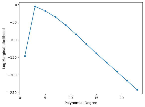
logML_values, mem_values, degrees = blr(N=15, gamma=1, basis='legendre', sigma=0.1)
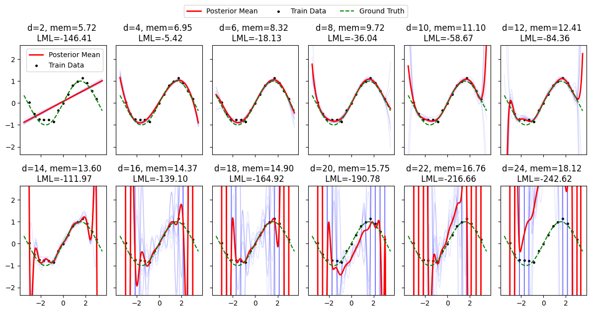
sns.lineplot(x=degrees, y=mem_values, marker='o')
plt.xlabel('Polynomial Degree')
plt.ylabel('Memorization (bits/param)')
plt.show()
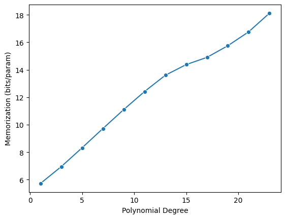
sns.lineplot(x=degrees, y=logML_values, marker='o')
plt.xlabel('Polynomial Degree')
plt.ylabel('Log Marginal Likelihood')
plt.show()
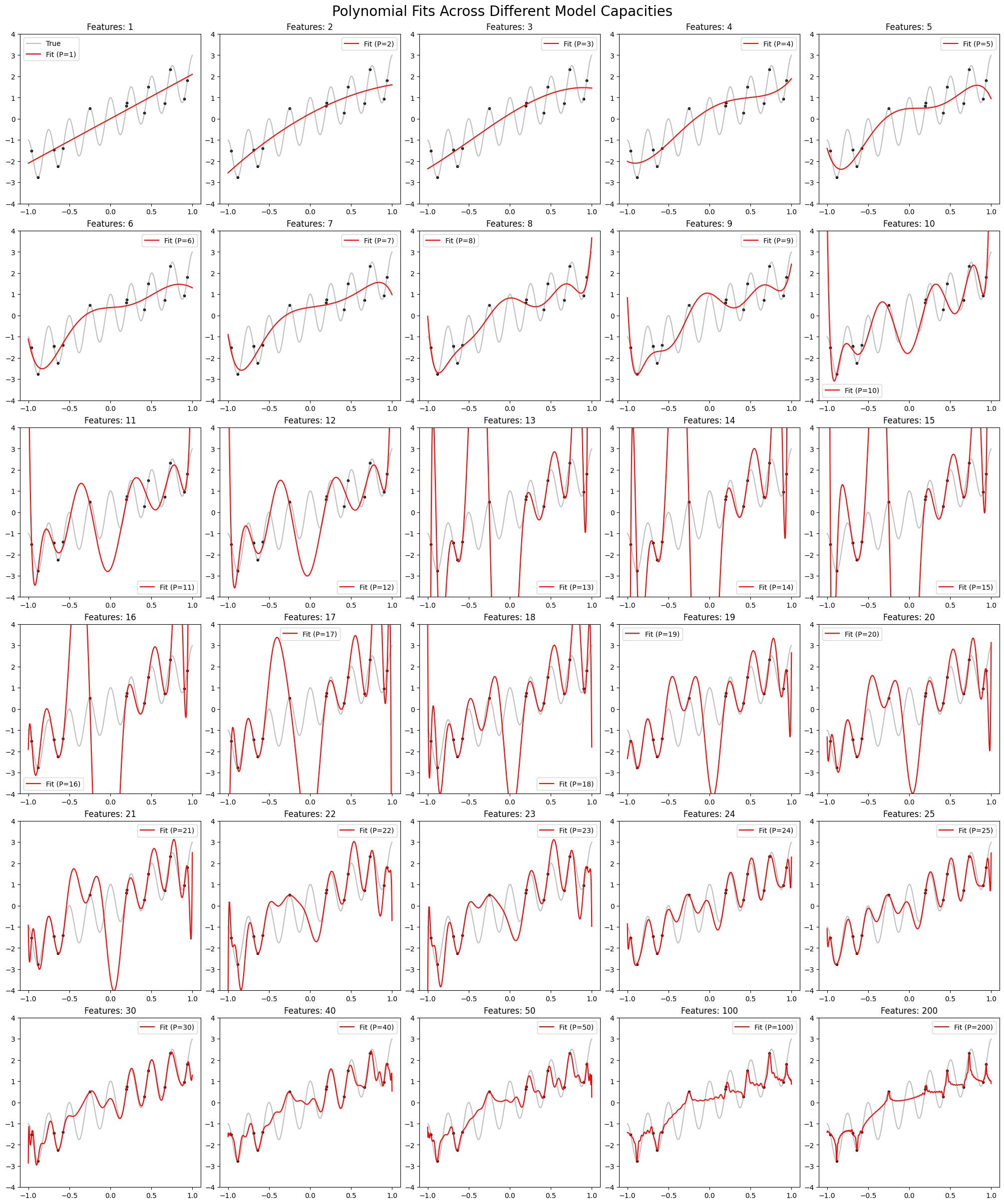
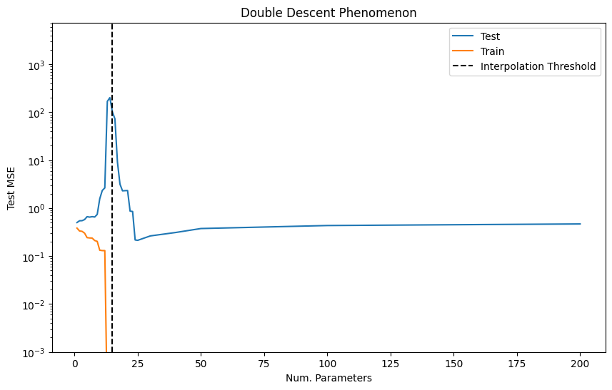
Double descent in polynomial regression
def compute_y_from_x(X: np.ndarray):
    return np.add(2.0 * X, np.cos(X * 25))[:, 0]

low, high = -1.0, 1.0
num_data = 15
num_features_list = [1, 2, 3, 4, 5, 6, 7, 8, 9, 10, 11, 12, 13, 14, 15,
                     16, 17, 18, 19, 20, 21, 22, 23, 24, 25, 30, 40, 50, 100, 200]

# Fixed training data for consistency across plots
np.random.seed(42)
X_train = np.random.uniform(low=low, high=high, size=(num_data, 1))
y_train = compute_y_from_x(X_train)

X_test = np.linspace(start=low, stop=high, num=1000).reshape(-1, 1)
y_test = compute_y_from_x(X_test)

mse_list = []
preds_list = [] # Store predictions for subplots

# --- Computations ---
for num_features in num_features_list:
    feature_degrees = 1 + np.arange(num_features).astype(int)

    # Fit using Legendre Polynomials
    X_train_poly = scipy.special.eval_legendre(feature_degrees, X_train)
    X_test_poly = scipy.special.eval_legendre(feature_degrees, X_test)
    #X_train_poly = np.vander(X_train.flatten(), num_features + 1, increasing=True)[:, 1:]
    #X_test_poly = np.vander(X_test.flatten(), num_features + 1, increasing=True)[:, 1:]

    # Solve via Moore-Penrose pseudoinverse
    beta_hat = np.linalg.pinv(X_train_poly) @ y_train

    y_train_pred = X_train_poly @ beta_hat
    y_test_pred = X_test_poly @ beta_hat

    mse_list.append({
        "Num. Parameters": num_features,
        "Train MSE": mean_squared_error(y_train, y_train_pred),
        "Test MSE": mean_squared_error(y_test, y_test_pred),
    })
    preds_list.append(y_test_pred)

# --- Visualization: Subplot Grid ---
n_plots = len(num_features_list)
cols = 5
rows = (n_plots // cols) + (1 if n_plots % cols != 0 else 0)

fig, axes = plt.subplots(rows, cols, figsize=(20, 4 * rows), constrained_layout=True)
axes = axes.flatten()

for i, num_features in enumerate(num_features_list):
    ax = axes[i]
    sns.lineplot(x=X_test[:, 0], y=y_test, ax=ax, color='gray', alpha=0.5, label="True" if i==0 else None)
    sns.lineplot(x=X_test[:, 0], y=preds_list[i], ax=ax, color='red', label=f"Fit (P={num_features})")
    sns.scatterplot(x=X_train[:, 0], y=y_train, ax=ax, s=20, color='black', edgecolor='white')

    ax.set_ylim(-4, 4)
    ax.set_title(f"Features: {num_features}")
    if i % cols != 0: ax.set_ylabel("")
    if i < (n_plots - cols): ax.set_xlabel("")

# Hide unused subplots
for j in range(i + 1, len(axes)):
    axes[j].axis('off')

plt.suptitle("Polynomial Fits Across Different Model Capacities", fontsize=20)
plt.show()

# --- Visualization: MSE Curves ---
mse_df = pd.DataFrame(mse_list)
plt.figure(figsize=(10, 6))
sns.lineplot(data=mse_df, x="Num. Parameters", y="Test MSE", label="Test")
sns.lineplot(data=mse_df, x="Num. Parameters", y="Train MSE", label="Train")
plt.axvline(x=num_data, color="black", linestyle="--", label="Interpolation Threshold")
plt.yscale("log")
plt.ylim(bottom=1e-3)
plt.title("Double Descent Phenomenon")
plt.legend()
plt.show()
np.random.seed(0)

def generate_data(N, noise_std=0.5):
    x = np.sort(np.random.uniform(-1, 1, size=N))
    y_true = np.sin(x * 5)
    y = y_true + np.random.normal(0, noise_std, size=N)
    return x, y, y_true

def basis_expansion(x, basis='legendre', poly_degree=3):
    if basis == 'linear':
        return np.vstack((np.ones_like(x), x)).T
    elif basis == 'polynomial':
        # Using Vandermonde: [x^0, x^1, ..., x^d]
        return np.vander(x, poly_degree + 1, increasing=True)
    elif basis == 'legendre':
        # Correctly evaluate Legendre polynomials for each degree
        X = np.zeros((len(x), poly_degree + 1))
        for d in range(poly_degree + 1):
            X[:, d] = scipy.special.eval_legendre(d, x)
        return X
    else:
        raise ValueError("Unknown basis")

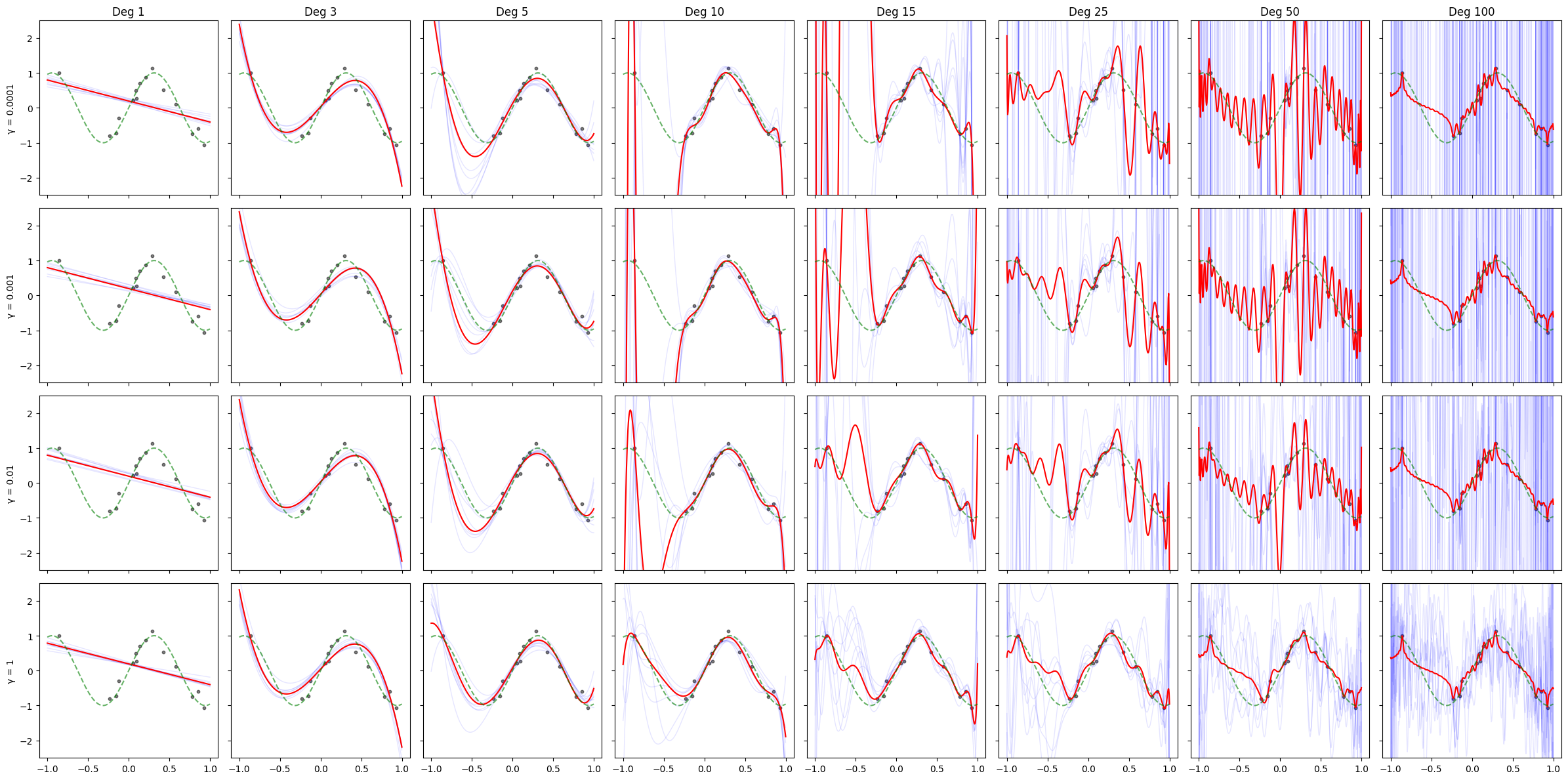
def blr_grid_analysis(N=15, sigma=0.2, basis='legendre'):
    x, y, y_true = generate_data(N, noise_std=sigma)
    degrees = [1, 3, 5, 10, 15, 25, 50, 100]
    gammas = [1e-4, 1e-3, 1e-2, 1]

    # Grid Plot Setup
    fig, axes = plt.subplots(len(gammas), len(degrees), figsize=(24, 12), sharex=True, sharey=True)

    results = []
    xtest = np.linspace(-1, 1, 400)
    ytest_true = np.sin(xtest * 5)

    for r, gamma in enumerate(gammas):
        for c, degree in enumerate(degrees):
            ax = axes[r, c]

            # Expansion
            X = basis_expansion(x, basis=basis, poly_degree=degree)
            Xtest = basis_expansion(xtest, basis=basis, poly_degree=degree)
            n, d = X.shape

            # Posterior
            S0_inv = gamma * np.eye(d)
            Sn_inv = S0_inv + (sigma**-2) * (X.T @ X)
            Sn = np.linalg.inv(Sn_inv)
            mn = Sn @ (sigma**-2 * X.T @ y)

            # --- Metrics ---
            y_train_pred = X @ mn
            y_test_pred = Xtest @ mn
            train_mse = mean_squared_error(y, y_train_pred)
            test_mse = mean_squared_error(ytest_true, y_test_pred)

            # Marginal Likelihood
            sse = np.sum((y - y_train_pred)**2)
            _, log_det_Sn_inv = np.linalg.slogdet(Sn_inv)
            log_ml = ((d/2) * np.log(gamma) - (n/2) * np.log(2 * np.pi) + n * np.log(1/sigma)
                      - 0.5 * log_det_Sn_inv - 0.5 * ((sigma**-2) * sse + gamma * (mn.T @ mn)))

            # Information Gain (KL Divergence)
            _, log_det_Sn = np.linalg.slogdet(Sn)
            log_det_S0 = -d * np.log(gamma)
            kl_div = 0.5 * (log_det_S0 - log_det_Sn + gamma * np.trace(Sn) + gamma * (mn.T @ mn) - d)
            bits_per_param = (kl_div / np.log(2)) / d

            results.append({
                "Gamma": gamma,
                "Degree": degree,
                "LML": log_ml,
                "Train MSE": train_mse,
                "Test MSE": test_mse,
                "Bits/Param": bits_per_param
            })

            # --- Plotting ---
            posterior_samples = np.random.multivariate_normal(mn, Sn, size=8)
            for w_post in posterior_samples:
                ax.plot(xtest, Xtest @ w_post, color='blue', alpha=0.1, lw=1)

            ax.plot(xtest, y_test_pred, color='red', lw=1.5)
            ax.scatter(x, y, color='black', s=10, alpha=0.5)
            ax.plot(xtest, ytest_true, color='green', ls='--', alpha=0.6)
            ax.set_ylim([-2.5, 2.5])

            if r == 0: ax.set_title(f'Deg {degree}')
            if c == 0: ax.set_ylabel(f'γ = {gamma}')

    plt.tight_layout()
    plt.show()
    df = pd.DataFrame(results)
    return df

N = 15
results_df = blr_grid_analysis(N=N, sigma=0.2, basis='legendre')
fig, (ax1, ax2) = plt.subplots(1, 2, figsize=(10, 3))
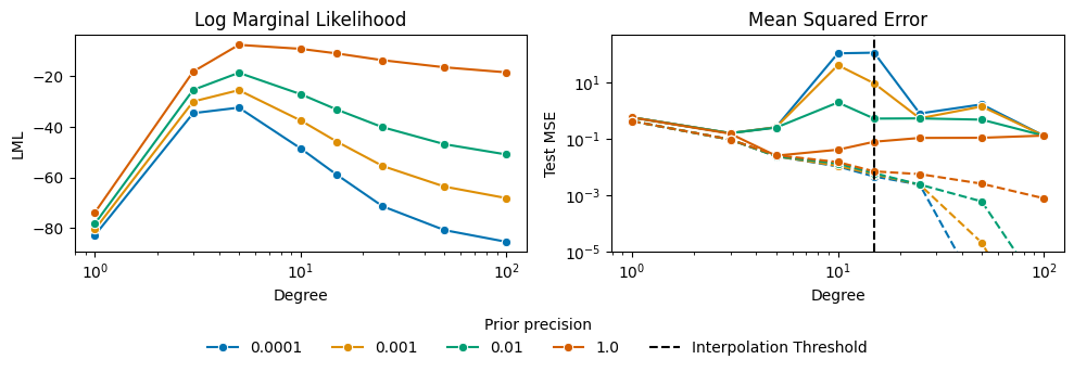
unique_gammas = results_df["Gamma"].nunique()
palette = sns.color_palette("colorblind", n_colors=unique_gammas)
# 1. Log Marginal Likelihood Plot
sns.lineplot(data=results_df, x="Degree", y="LML", hue="Gamma", marker="o", ax=ax1, palette=palette, legend=None)
ax1.set_title("Log Marginal Likelihood")
ax1.set_xscale("log")

# 2. Test MSE Plot (Double Descent)
sns.lineplot(data=results_df, x="Degree", y="Test MSE", hue="Gamma", marker="o", ax=ax2, palette=palette)
sns.lineplot(data=results_df, x="Degree", y="Train MSE", hue="Gamma", marker="o", linestyle='--', ax=ax2, palette=palette, legend=None)
ax2.set_title("Mean Squared Error")
ax2.set_yscale("log")
ax2.set_xscale("log")
ax2.set_ylim(bottom=1e-5)
ax2.axvline(x=N, color='black', linestyle='--', label='Interpolation Threshold')


handles, labels = ax2.get_legend_handles_labels()
ax2.get_legend().remove() # Remove the default legend from inside the plot

fig.legend(handles, labels, loc='lower center', title='Prior precision', ncol=len(labels),
           bbox_to_anchor=(0.5, -0.15), frameon=False)

plt.tight_layout()
plt.show()
References
[1] Schaeffer, Rylan, et al. “Double descent demystified: Identifying, interpreting & ablating the sources of a deep learning puzzle.” arXiv preprint arXiv:2303.14151 (2023).